
NALO-VOM: Navigation-Oriented LiDAR-Guided Monocular Visual Odometry and Mapping
📌 Overview
Traditional monocular visual odometry (VO) often struggles with sparse environment maps that lack the structural detail necessary for autonomous vehicle navigation. To address this, we propose NALO-VOM, a system that transfers the geometric structural knowledge of 3D LiDAR to a monocular VO framework via an offline-trained major-plane prediction network. By utilizing non-artificial projection labels during training, the system enables a single camera to predict major-plane masks (MP-Masks) in real-time. This integration allows for scale-consistent camera pose estimation and the reconstruction of semi-dense maps that are high-quality and dense enough to be transformed into 2D grid maps for motion planning. Extensive experiments on the KITTI dataset and real-world platforms demonstrate that NALO-VOM achieves superior localization accuracy and provides a reliable mapping solution for obstacle avoidance and decision-making in UGV navigation.
🚀 Key Contributions
- LiDAR-to-Camera Knowledge Transfer: We pioneered a method to transfer the structural representation ability of 3D LiDAR to a monocular VO system using a major-plane prediction network.
- Major-Plane Mask (MP-Mask) Integration: The network predicts an MP-Mask for each image frame to assist in dense front-end tracking and ground plane extraction.
- Scale Optimization: By leveraging the extracted ground plane, the system significantly constrains scale drift, a common issue in long-term monocular VO.
- Semi-Dense Mapping: Major planes are incorporated to build a high-quality map capable of supporting UGV motion planning and decision-making.
🛠️ System Architecture & Methodology
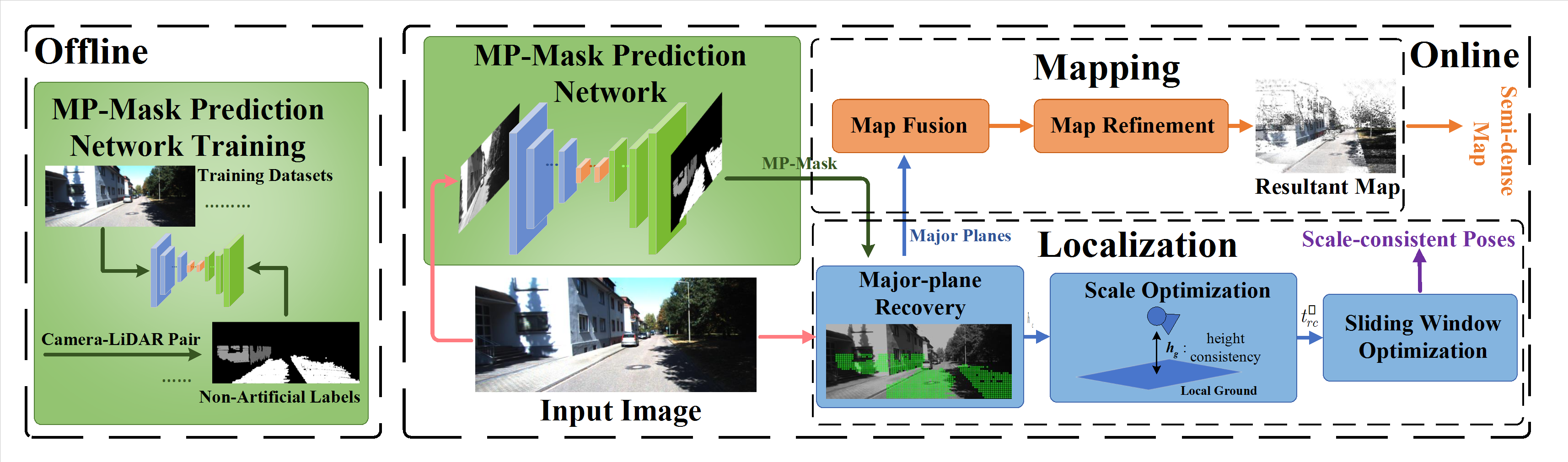 The system architecture of NALO-VOM
Our framework consists of two main phases: an offline LiDAR-guided training process and an online monocular odometry process.
1. Offline Major-Plane Prediction Network
- We utilize a ResNet-50-based architecture to predict major planes (e.g., ground, walls) that possess uniform planar curvature and occupy large areas.
- The network is trained offline using non-artificial projection labels generated by perfectly synchronized camera-LiDAR pairs.
- The training loss \(E(g)\) is formulated as a sum of the variance and a weighted squared mean of the error in log space: \(E(g)=\frac{1}{c}\sum_{i=0}^{h}\sum_{j=0}^{w}g_{(i,j)}^{2}-\frac{\lambda}{c^{2}}(\sum_{i=0}^{h}\sum_{j=0}^{w}g_{(i,j)})^{2}\)
2. Online Dense Tracking & Scale Optimization
Dense Tracking: During the online phase, the system only takes RGB images as inputs. The network generates an MP-Mask, which provides additional depth pixels for robust front-end tracking. For a point on a fitted plane parameterized by \(\pi=[\vec{n}^{T},\sigma]^{T}\), the newly added depth \(d_{p}^{*}\) is given by: \(d_{p}^{*}=\vec{n}^{T}\cdot K^{-1}\cdot p\cdot\sigma^{-1}\)
Photometric Optimization: The system minimizes the photometric error across a sliding window of length \(W\). The loss function is defined as: \(\mathcal{L} = \text{arg min}_{\xi_r, \xi_t, \Theta_{id}} \sum_{r=1}^W \sum_{t=1}^W \sum_{p \in N_r} \omega_p ||I_t(p') - I_r(p)||_{\gamma} \quad (3)\) where the weighting factor \(\\omega_p\) handles gradient consistency: \(\\omega_p = \frac{m^2}{m^2 + ||\nabla I_r(p)||_2^2} \quad (4)\)
Projection Model: The projected point position \(p'\) is derived via the transformation matrix: \(P_t = \begin{bmatrix} x \\ y \\ z \end{bmatrix} = R(d_p^{-1} K^{-1} p) + t \quad (5)\) \(T_{tr} = \begin{bmatrix} R & t \\ 0 & 1 \end{bmatrix} \quad (6)\)
Depth Estimation & Uncertainty: The inverse depth \(d_p\) is calculated using the matching point \(u_m\) on the epipolar line: \(d_p = \frac{x_{pc} - u_m z_{pc}}{u_m z_t - x_t} \quad (7)\) To account for noise, we define the search range \((d_p^{min}, d_p^{max})$ using the uncertainty $\sigma_{\lambda}\): \(d_p^{min} = \frac{x_{pc} - (u_m + \sigma_{\lambda}) z_{pc}}{(u_m + \sigma_{\lambda}) z_t - x_t}, \quad d_p^{max} = \frac{x_{pc} - (u_m - \sigma_{\lambda}) z_{pc}}{(u_m - \sigma_{\lambda}) z_t - x_t} \quad (8, 9)\)
Scale Recovery: Assuming a constant vertical distance \(h_g\) between the camera and the local ground, we impose a scale constraint \(\rho_c = h_g / h_c\) to update the translation vectors and perform sliding window optimization.
3. Semi-Dense Map Reconstruction
- To reconstruct texture-less areas without relying on computationally heavy pixel-wise depth networks, we introduce major-planes into the map building process.
- The major-planes are aligned to the nearest planes in the sparse point cloud map using the following loss function: \(\mathcal{L}_{k}=\sum_{p\in^{n}\pi_{k}}\frac{||^{n}\pi_{k}^{DSO^{T}}\cdot p||_{2}}{nN_{k}}\)
- This combination of sparse feature points and major-planes yields a dense environment map that accurately represents the environment’s geometry.
📊 Experimental Results
1. Localization Accuracy (KITTI Dataset)
On the KITTI dataset, NALO-VOM outperformed state-of-the-art methods (like ORB-SLAM2 and DSO), achieving the lowest translation error on 8 out of 11 sequences.
| Seq | ORB-SLAM2 [9] | DSO [3] | Song et.al [40] | Wang et.al [19] | Ours |
|---|---|---|---|---|---|
| Trans (%) / Rot (deg/m) | |||||
| 00 | 28.84 / 0.1982 | 29.78 / 0.2023 | 2.04 / 0.0048 | 1.01 / 0.0014 | 1.19 / 0.0028 |
| 01 | * | 1.79 / 0.0014 | - | - | 1.11 / 0.0009 |
| 02 | 2.63 / 0.0016 | 5.43 / 0.0038 | 1.50 / 0.0035 | 0.93 / 0.0018 | 1.91 / 0.0029 |
| 03 | 1.12 / 0.0020 | 0.79 / 0.0021 | 3.37 / 0.0021 | 0.52 / 0.0010 | 0.82 / 0.0021 |
| 04 | 2.25 / 0.0018 | 0.89 / 0.0021 | 2.19 / 0.0028 | 1.16 / 0.0023 | 0.85 / 0.0020 |
| 05 | 8.53 / 0.0055 | 7.80 / 0.0015 | 1.43 / 0.0038 | 1.45 / 0.0014 | 1.01 / 0.0015 |
| 06 | 18.21 / 0.0074 | 18.08 / 0.0019 | 2.09 / 0.0081 | 2.92 / 0.0027 | 1.33 / 0.0019 |
| 07 | 9.60 / 0.0121 | 7.52 / 0.0038 | - | 1.73 / 0.0023 | 1.59 / 0.0036 |
| 08 | 12.39 / 0.0032 | 8.36 / 0.0028 | 2.37 / 0.0044 | 1.18 / 0.0017 | 0.90 / 0.0021 |
| 09 | 16.64 / 0.0053 | 9.54 / 0.0019 | 1.76 / 0.0047 | 1.17 / 0.0020 | 1.02 / 0.0022 |
| 10 | 5.07 / 0.0063 | 5.49 / 0.0034 | 2.12 / 0.0085 | 0.93 / 0.0029 | 0.85 / 0.0025 |
| Avg | 10.53 / 0.0243 | 8.68 / 0.0206 | 2.10 / 0.0047 | 1.25 / 0.0020 | 1.14 / 0.0022 |
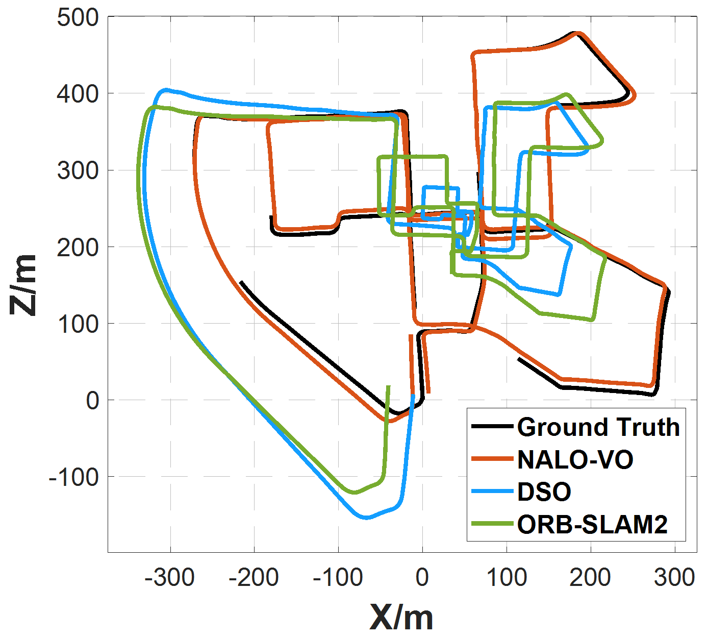
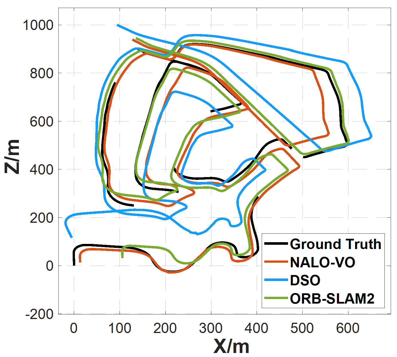
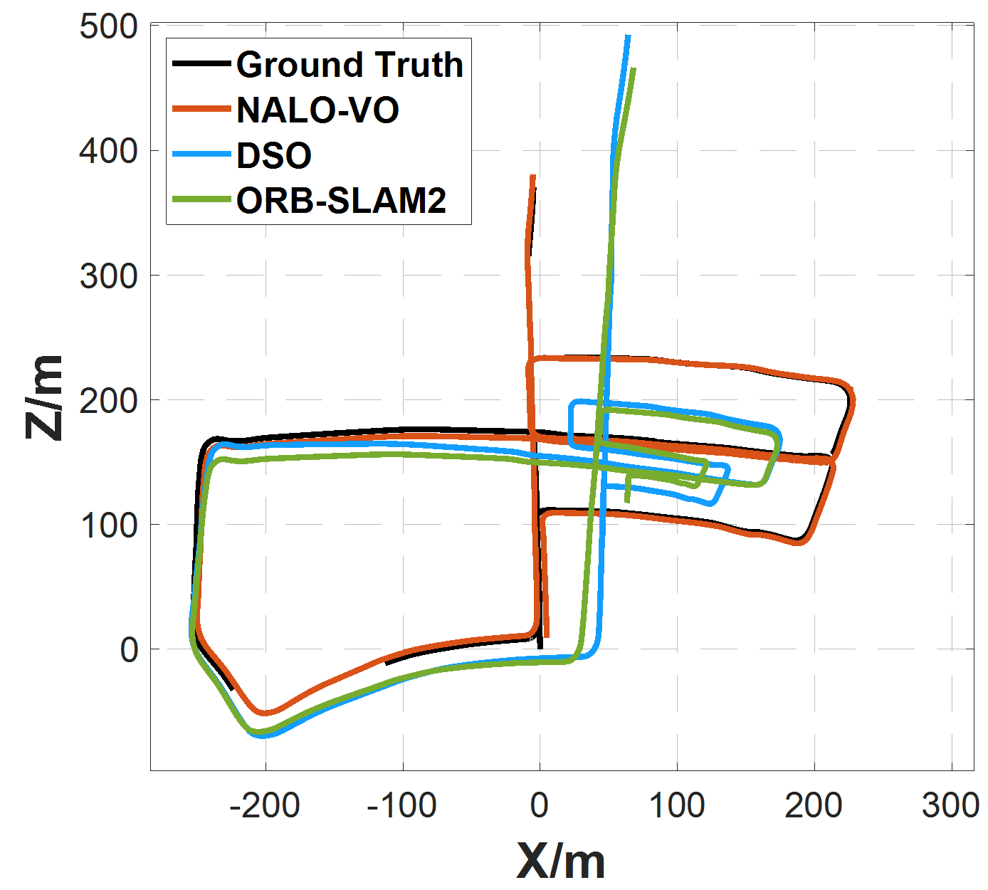
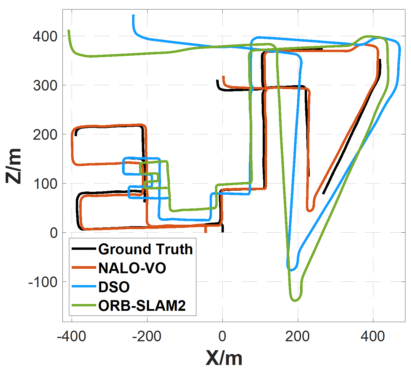
(Caption: Trajectory comparison on KITTI sequences 00, 02, 05, and 08. NALO-VO (red) stays closest to the ground truth (black).)
2. Mapping Density & Quality
The point densities of critical driving-aware objects built by NALO-VOM greatly exceed those built by baseline methods.
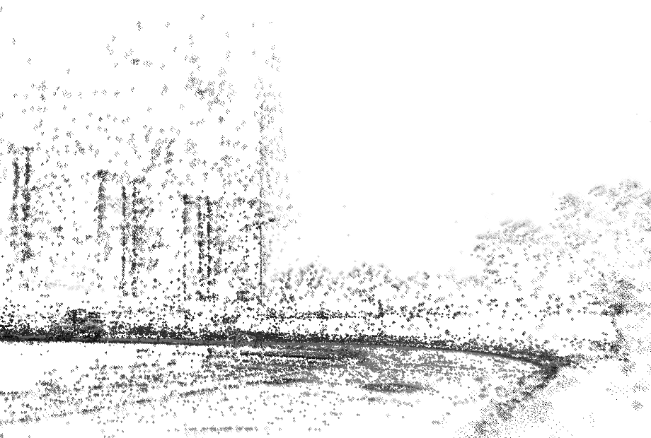
Standard DSO Mapping (Sparse)
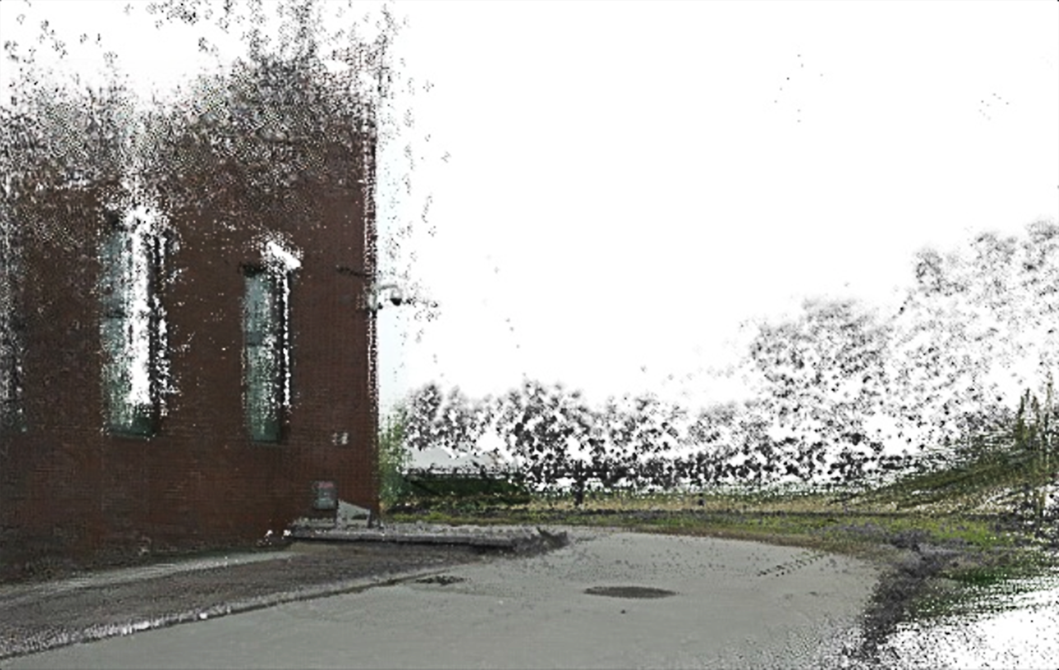
NALO-VOM Mapping (Ours, Semi-dense)
(Caption: Comparison of mapping density in a real-world scenario. NALO-VOM provides a much denser semi-dense point cloud suitable for navigation.)
3. Navigation Applicability
We successfully projected the semi-dense 3D point cloud into a 2D navigation grid map. Using the Hybrid A* algorithm, we proved that our map enables valid path planning and obstacle avoidance for UGVs.
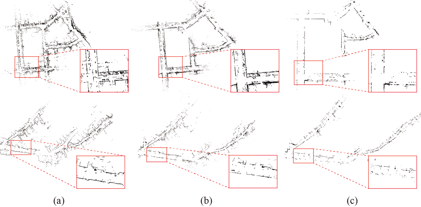
Fig 7: 2D Grid Map Comparison
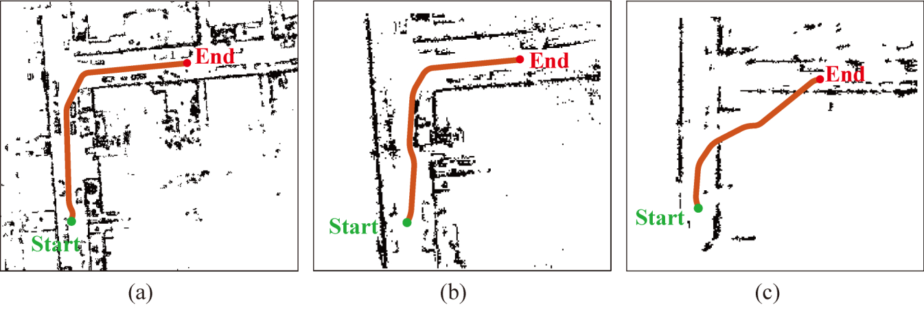
Fig 8: Hybrid A* Path Planning
4. Real-World Deployment
The system was successfully deployed on real-world UGV platforms, running at ~14 FPS on an NVIDIA RTX 3070, demonstrating excellent generalization and real-time capability.
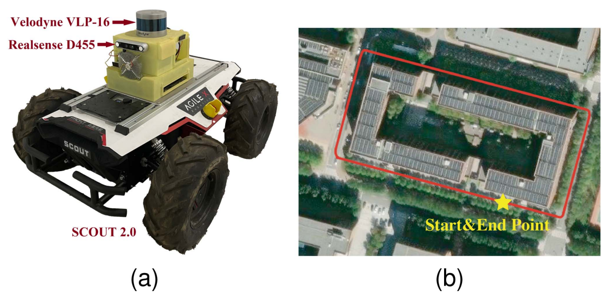
(a) Scout 2.0 Platform & Test Area
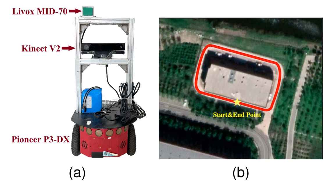
(b) Pioneer P3-DX Platform & Test Area
We evaluated NALO-VOM in various outdoor environments. The system maintained stable tracking and produced high-quality maps even in challenging conditions.
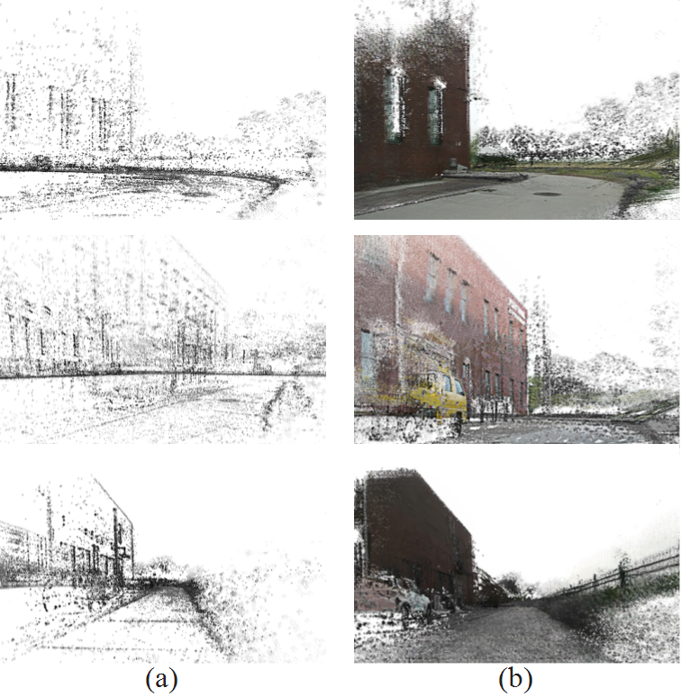
Comparison of real-world mapping results in different campus scenarios.