
BCS-Tool
BCS-Tool
Size battery storage for an entire industrial park in seconds. Give it a year of net-load data and get the optimal capacity, dispatch schedule and annual savings, plus payback period, NPV and IRR.
Why BCS-Tool
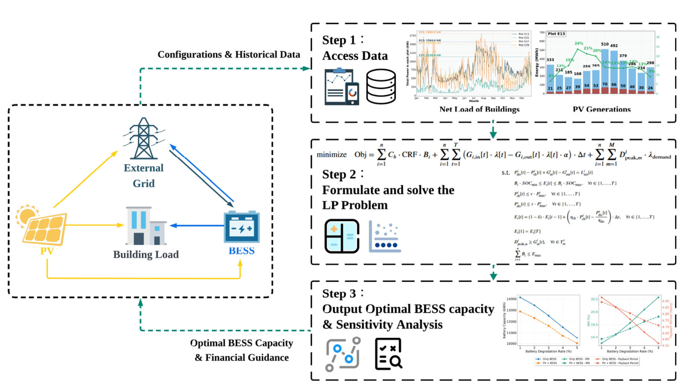
Battery sizing studies usually rely on mixed-integer models that are slow, or on rule-based control that leaves savings on the table. BCS-Tool solves sizing and year-round dispatch together as one linear program.
Fast, exact optimum
No binary variables. The pure LP reaches the same capacity as the MILP benchmark, about 13.6 times faster.
Sizing and dispatch together
Capacity and every time step of charging and discharging are optimized at once, so the result reflects the best possible operation.
Investment-ready metrics
Reports annual savings, payback period, NPV and IRR, with the battery cost annualized over the project life.
Real tariffs
Hourly time-of-use prices or seasonal peak, high, flat and valley tiers, plus monthly or daily demand charges and export credits.
Multi-site allocation
Split one storage budget across several sub-plots, each with its own meter and load, in a single joint optimization.
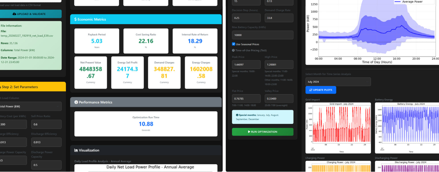
Python API and web interface
Script batch studies and sensitivity analyses in Python. A Flask browser interface with charts is included in the repository.
How it works
- Bring your dataA CSV of net load (building load minus PV) with a timestamp column. One full year at 15-min to 1-h resolution is recommended.
- Set the economicsBattery cost, efficiencies, state-of-charge limits, power ratio, tariff, demand charge, export price ratio, discount rate and project life.
- OptimizeThe LP returns the optimal capacity, the full charging schedule, grid import and export, and the financial indicators.
Proven on a real industrial park
Four sub-plots and 59 enterprises in Changsha, China, with one year of 15-min smart-meter load data and 2.1 MW of simulated rooftop and facade PV.
| Result | Value |
|---|---|
| Optimal storage, sized per sub-plot (one-part / two-part tariff) | 16,359 / 11,373 kWh |
| Payback, storage only, every sub-plot | within 3.6 years |
| Whole park with PV + storage, 10 MWh budget (one-part tariff) | 4.56 yr payback · 20.63% IRR |
| Solve time, LP vs. MILP (single-thread) | 8.60 s vs. 116.80 s |
| Capacity suggested by rule-based sizing for comparison (one-part tariff) | 5,959 kWh |
Get started
Python 3.8 or later and a Gurobi license (free for academic use) are required.
# 1. Clone and install
git clone https://github.com/huziqi/BCS-Tool.git
cd BCS-Tool
pip install -e .
pip install matplotlib numpy-financial flask flask-cors

# 2. Activate your Gurobi license: https://www.gurobi.com/academia/
from pvbat_optimizer import PVBatOptimizer_linearProg, OptimizerConfig, OptimizerUtils

# CSV: first column is a timestamp, second is net load in kW
net_load = OptimizerUtils.net_profiles("net_load.csv")

config = OptimizerConfig(
    battery_cost_per_kwh=1000,        # CNY/kWh
    use_seasonal_prices=True,        # peak / high / flat / valley tariff
    demand_charge_rate=33.8,
    years=15, discount_rate=0.12,
    decision_step=0.25,                # hours per time step (15-min data)
)

result = PVBatOptimizer_linearProg(config).optimize(net_load)
print(result["battery_capacity"], result["annual_savings"])

# Payback period, NPV and IRR
metrics = OptimizerUtils.calculate_economic_metrics(
    annual_savings=result["annual_savings"],
    project_lifetime=config.years,
    discount_rate=config.discount_rate,
    battery_construction_cost=result["battery_construction_cost"],
)
from pvbat_optimizer import MultiPlotOptimizer

loads = {"E13": load_e13, "E25": load_e25}   # pandas Series on the same time index
res = MultiPlotOptimizer(config, total_battery_capacity=10000).optimize_multi_plots(loads)
print(res["capacity_allocation"])
python app.py # serves the interface at http://localhost:5000Cite
Figures reproduced from the open-access article under CC BY 4.0.